A model should be as simple as possible, but no simpler – Albert Einstein
Various tools for Prediction and/or Description goals in regression, classification and machine learning.
Some of them are associated with my book, From Linear Models to Machine Learning: Statistical Regression and Classification, N. Matloff, CRC, 2017 (recipient of the Eric Ziegel Award for Best Book Reviewed in 2017, Technometrics), and with my forthcoming book, The Art of Machine Learning: Algorithms+Data+R, NSP, 2020 . But the tools are useful in general, independently of the books.
CLICK HERE for a regtools Quick Start!
See full function list by typing
> ?regtoolsHere are the main categories:
Here we will take a quick tour of a subset of regtools features, using datasets mlb and prgeng that are included in the package.
The mlb dataset consists of data on Major Leage baseball players. We’ll use only a few features, to keep things simple:
> data(mlb)
> head(mlb)
             Name Team       Position Height
1   Adam_Donachie  BAL        Catcher     74
2       Paul_Bako  BAL        Catcher     74
3 Ramon_Hernandez  BAL        Catcher     72
4    Kevin_Millar  BAL  First_Baseman     72
5     Chris_Gomez  BAL  First_Baseman     73
6   Brian_Roberts  BAL Second_Baseman     69
  Weight   Age PosCategory
1    180 22.99     Catcher
2    215 34.69     Catcher
3    210 30.78     Catcher
4    210 35.43   Infielder
5    188 35.71   Infielder
6    176 29.39   Infielder
We’ll predict player weight (in pounds) and position.
The prgeng dataset consists of data on Silicon Valley programmers and engineers in the 2000 US Census. It is available in several forms. We’ll use the data frame version, and againn use only a few features to keep things simple:
> data(peFactors)
> names(peFactors)
 [1] "age"      "cit"      "educ"     "engl"     "occ"      "birth"
 [7] "sex"      "wageinc"  "wkswrkd"  "yrentry"  "powspuma"
> pef <- peFactors[,c(1,3,5,7:9)]
> head(pef)
       age educ occ sex wageinc wkswrkd
1 50.30082   13 102   2   75000      52
2 41.10139    9 101   1   12300      20
3 24.67374    9 102   2   15400      52
4 50.19951   11 100   1       0      52
5 51.18112   11 100   2     160       1
6 57.70413   11 100   1       0       0
The various education and occupation codes may be obtained from the reference in the help page for this dataset.
We’ll predict wage income. One cannot get really good accuracy with the given features, but this dataset will serve as a good introduction to these particular features of the package.
NOTE: The qe-series functions have been spun off to a separate package, ##qeML##.
The qe*() functions’ output are ready for making prediction on new cases. We’ll use this example:
> newx <- data.frame(age=32, educ='13', occ='106', sex='1', wkswrkd=30)One of the features of regtools is its qe*() functions, a set of wrappers. Here ‘qe’ stands for “quick and easy.” These functions provide convenient access to more sophisticated functions, with a very simple, uniform interface.
Note that the simplicity of the interface is just as important as the uniformity. A single call is all that is needed, no preparatory calls such as model definition.
The idea is that, given a new dataset, the analyst can quickly and easily try fitting a number of models in succession, say first k-Nearest Neighbors, then random forests:
# fit models
> knnout <- qeKNN(mlb,'Weight',k=25)
> rfout <- qeRF(mlb,'Weight')

# mean abs. pred. error on holdout set, in pounds
> knnout$testAcc
[1] 11.75644
> rfout$testAcc
[1] 12.6787

# predict a new case
> newx <- data.frame(Position='Catcher',Height=73.5,Age=26)
> predict(knnout,newx)
       [,1]
[1,] 204.04
> predict(rfout,newx)
      11
199.1714
How about some other ML methods?
> lassout <- qeLASSO(mlb,'Weight')
> lassout$testAcc
[1] 14.23122

# poly regression, degree 3
> polyout <- qePolyLin(mlb,'Weight',3)
> polyout$testAcc
[1] 13.55613

> nnout <- qeNeural(mlb,'Weight')
# ...
> nnout$testAcc
[1] 12.2537
# try some nondefault hyperparams
> nnout <- qeNeural(mlb,'Weight',hidden=c(200,200),nEpoch=50)
> nnout$testAcc
[1] 15.17982
More about the series
They automatically assess the model on a holdout set, using as loss Mean Absolute Prediction Error or Overall Misclassification Rate. (Setting holdout = NULL turns off this option.)
They handle R factors correctly in prediction, which some of the wrapped functions do not do by themselves (more on this point below).
Call form for all qe*() functions:
qe*(data,yName, options incl. method-specific)Currently available:
qeLin() linear model, wrapper for lm()
qeLogit() logistic model, wrapper for glm(family=binomial)
qeKNN() k-Nearest Neighbors, wrapper for the regtools function kNN()
qeRF() random forests, wrapper for randomForest package
qeGBoost() gradient boosting on trees, wrapper for gbm package
qeSVM() SVM, wrapper for e1071 package
qeNeural() neural networks, wrapper for regtools function krsFit(), in turn wrapping keras package
qeLASSO() LASSO/ridge, wrapper for glmnet package
qePolyLin() polynomial regression, wrapper for the polyreg package, providing full polynomial models (powers and cross products), and correctly handling dummy variables (powers are not formed)
qePolyLog() polynomial logistic regression
The classification case is specified by there being an R factor in the second argument.
Quick and easy comparison of several ML methods on the same data, e.g.:
qeCompare(mlb,'Weight',
   c('qeLin','qePolyLin','qeKNN','qeRF','qeLASSO','qeNeural'),25)
#       qeFtn  meanAcc
# 1     qeLin 13.30490
# 2 qePolyLin 13.33584
# 3     qeKNN 13.72708
# 4      qeRF 13.46515
# 5   qeLASSO 13.27564
# 6 qeNeural 14.01487 Seamless incorporation of PCA dimension reduction into qe methods, e.g.
z <- pcaQE(0.6,d2,'tot','qeKNN',k=25,holdout=NULL)
newx <- d2[8,-13]
predict(z,newx)
#         [,1]
# [1,] 1440.44Actual calls in the qe*-series functions.
# qeKNN()
regtools::kNN(xm, y, newx = NULL, k, scaleX = scaleX, classif = classif)
# qeRF()
randomForest::randomForest(frml,
   data = data, ntree = nTree, nodesize = minNodeSize)
# qeSVM()
e1071::svm(frml, data = data, cost = cost, gamma = gamma, decision.values = TRUE)
# qeLASSO()
glmnet::cv.glmnet(x = xm, y = ym, alpha = alpha, family = fam)
# qeGBoost()
gbm::gbm(yDumm ~ .,data=tmpDF,distribution='bernoulli',  # used as OVA
         n.trees=nTree,n.minobsinnode=minNodeSize,shrinkage=learnRate)
# qeNeural()
regtools::krsFit(x,y,hidden,classif=classif,nClass=length(classNames),
      nEpoch=nEpoch)  # regtools wrapper to keras package
# qeLogit()
glm(yDumm ~ .,data=tmpDF,family=binomial)  # used with OVA
# qePolyLin()
regtools::penrosePoly(d=data,yName=yName,deg=deg,maxInteractDeg)
# qePolyLog()
polyreg::polyFit(data,deg,use="glm")So, let’s try that programmer and engineer dataset.
> lmout <- qeLin(pef,'wageinc')
> lmout$testAcc
[1] 25520.6 # Mean Absolute Prediction Error on holdout set
> predict(lmout,newx)
11
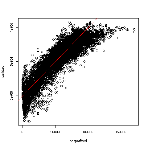
35034.63 The fit assessment techniques in regtools gauge the fit of parametric models by comparing to nonparametric ones. Since the latter are free of model bias, they are very useful in assessing the parametric models. One of them plots parametric vs. k-NN fit:
> parvsnonparplot(lmout,qeKNN(pef,'wageinc',25))We specified k = 25 nearest neighbors. Here is the plot:
Glancing at the red 45-degree line, we see some suggestion here that the linear model tends to underpredict at low and high wage values. If the analyst wished to use a linear model, she would investigate further (always a good idea before resorting to machine learning algorithms), possibly adding quadratic terms to the model.
We saw above an example of one such function, parvsnonparplot(). Another is nonparvarplot(). Here is the data prep:
data(peDumms)  # dummy variables version of prgeng
pe1 <- peDumms[c('age','educ.14','educ.16','sex.1','wageinc','wkswrkd')]
We will check the classical assumption of homoscedasticity, meaning that the conditional variance of Y given X is constant. The function nonparvarplot() plots the estimated conditional variance against the estimated conditional mean, both computed nonparametrically:

Though we ran the plot thinking of the homoscedasticity assumption, and indeed we do see larger variance at large mean values, this is much more remarkable, showing that there are interesting subpopulations within this data. Since there appear to be 6 clusters, and there are 6 occupations, the observed pattern may reflect this.
The package includes various other graphical diagnostic functions, such asnonparvsxplot().
By the way, violation of the homoscedasticity assumption won’t invalidate the estimates in our linear model. They still will be statistically consistent. But the standard errors we compute, and thus the statistical inference we perform, will be affected. This is correctible using the Eicker-White procedure, which for linear models is available in the car and sandwich packages. Our package here also extends this to nonlinear parametric models, in our function nlshc() (the validity of this extension is shown in the book).
Many statistical/machine learning methods have a number of tuning parameters (or hyperparameters). The idea of a grid search is to try many combinations of candidate values of the tuning parameters to find the “best” combination, say in the sense of highest rate of correct classification in a classification problem.
A number of machine learning packages include grid search functions. But the one in regtools has some novel features not found in the other packages:
Use of standard errors to avoid “p-hacking.”
A graphical interface, enabling the user to see at a glance how the various hyperparameters interact.
First, though, a brief discussion regardng finding the “best” hyperparameter combination.
But why the quotation marks around the word best above? The fact is that, due to sampling variation, a naive grid search may not give you the best parameter combination, due to sampling variation:
The full dataset is a sample from some target population.
Most grid search functions use cross-validation, in which the data are (one or more times) randomly split into a training set and a prediction set, thus adding further sampling variation.
So the parameter combination that seems best in the grid search may not actually be best. It may do well just by accident, depending on the dataset size, the number of cross-validation folds, the number of features and so on.
In other words:
Grid search is actually a form of p-hacking.
Thus one should not rely on the “best” combination found by a grid search. One should consider several combinations that did well. A good rule is that if several combinations yield about the same result, one should NOT necessarily choose the combination with the absolute minimum loss; one might instead just the one with the smallest standard error, as it’s the one we’re most sure of.
And moreover…
In fact, it is often wrong to even speak of the “best” hyperparameter combination in the first place. This is because there actually might be several optimal configurations, due to the fact that the mean loss sample loss values of different hyperparameters may be correlated often negatively. Thus we should not be surprised when we see several configurations that are quite different from each other yet have similar loss values.
Just pick a good combination of hyperparameters, without obsessing too much over “best,” and pay attention to standard errors.
The regtools grid search function fineTuning() is an advanced grid search tool, in two ways:
It aims to counter p-hacking, by forming Bonferoni-Dunn confidence intervals for the mean losses.
It provides a plotting capability, so that the user can see at a glance which several combinations of parameters look promising, thereby providing guidance for further combinations to investigate.
Here is an example using the famous Pima diabetes data (stored in a data frame db in the example below). This is a binary problem in which we are predicting presence or absence of the disease. We’ll do an SVM analysis, with our hyperparameters being gamma, a shape parameter, and cost, the penalty for each datapoint inside the margin.
The regtools grid search function fineTuning() calls a user-defined function that fits the user’s model on the training data and then predicts on the test data. The user-defined function is specified in the fineTuning() argument regcall, which in our example here will be pdCall:
# user provides a function stating the analysis to run on any parameter
# combination cmbi; here dtrn and dtst are the training and test sets,
# generated by fineTuning()

> pdCall <- function(dtrn,dtst,cmbi) {
   # fit training set
   svmout <-
      qeSVM(dtrn,'occ',gamma=cmbi$gamma,cost=cmbi$cost,holdout=NULL)
   # predict test set
   preds <- predict(svmout,dtst[,-3])$predClasses
   # find rate of correct classification
   mean(preds != dtst$occ)
}

> ftout <- fineTuning(dataset=pef,pars=list(gamma=c(0.5,1,1.5),cost=c(0.5,1,1.5)),regCall=pdCall,nTst=50,nXval=10)
And the output:
> ft$outdf
> ftout$outdf
  gamma cost meanAcc      seAcc    bonfAcc
1   0.5  1.5   0.570 0.03296463 0.09140832
2   1.0  1.0   0.576 0.02061283 0.05715776
3   0.5  0.5   0.582 0.02393510 0.06637014
4   1.5  1.5   0.594 0.02045048 0.05670758
5   1.5  0.5   0.608 0.01936779 0.05370534
6   0.5  1.0   0.608 0.02274496 0.06306999
7   1.5  1.0   0.608 0.02908990 0.08066400
8   1.0  0.5   0.614 0.01550627 0.04299767
9   1.0  1.5   0.626 0.01790096 0.04963796
Here is what happened in the fineTuning() call:
We fit SVM models, using qeSVM(), which has two SVM-specific parameters, gamma and cost. (See the documentation for e1071::svm().)
We specified the values 0.5, 1 and 1.5 for gamma, and the same for cost. That means 9 possible combinations.
The function fineTuning() generated those 9 combinations, running qeSVM() on each one,
Running qeSVM() is accomplished via the fineTuning() argument regCall, which specifies a user-written function, in this case pdCall().
In calling regCall(), fineTuning() passes the current hyperparameter combination, cmbi, and the current training and holdout sets, dtrn and dtst. The user-supplied regCall(), in this case pdCall() then calls the desired machine learning function, here qeSVM(), and calculates the resulting mean loss for that combination.
Technically the best combination is (0.5,1.5), but several gave similar results, as can be seen by the Bonferroni-Dunn column, which gives radii of approximate 95% confidence intervals. A more thorough investigation would involve a broader range of values for gamma and cost.
The corresponding plot function, called simply as
plot(ftout)uses the notion of parallel coordinates. The plot, not shown here, has three vertical axes, represent gamma, cost and meanAcc from the above output. Each polygonal line represents one row from outdf above, connecting the values of the three variables.
This kind of plot is most useful when we have several hyperparameters, not just 2 as in the current setting. It allows one to see at a glance which hyperparameter combinations.
The LetterRecognition dataset in the mlbench package lists various geometric measurements of capital English letters, thus another image recognition problem. One problem is that the frequencies of the letters in the dataset are not similar to those in actual English texts. The correct frequencies are given in the ltrfreqs dataset included here in the regtools package.
We can adjust the analysis accordingly, using the classadjust() function.
This allows use of ordinary tools like lm() for prediction in time series data. Since the goal here is prediction rather than inference, an informal model can be quite effective, as well as convenient. Note that we can also use the machine learning functions.
The basic idea is that x[i] is predicted by x[i-lg], x[i-lg+1], x[i-lg+2], i… x[i-1], where lg is the lag.
> xy <- TStoX(Nile,5)
> head(xy)
#      [,1] [,2] [,3] [,4] [,5] [,6]
# [1,] 1120 1160  963 1210 1160 1160
# [2,] 1160  963 1210 1160 1160  813
# [3,]  963 1210 1160 1160  813 1230
# [4,] 1210 1160 1160  813 1230 1370
# [5,] 1160 1160  813 1230 1370 1140
# [6,] 1160  813 1230 1370 1140  995
> head(Nile,36)
#  [1] 1120 1160  963 1210 1160 1160  813 1230 1370 1140  995  935 1110  994 1020
# [16]  960 1180  799  958 1140 1100 1210 1150 1250 1260 1220 1030 1100  774  840
# [31]  874  694  940  833  701  916
Try qeLin(). We’ll need to convert to data frame form for this:
> xyd <- data.frame(xy)  # col names now X1,...,X6
> lmout <- qeLin(xyd,'X6')
> lmout
> lmout
...
Coefficients:
(Intercept)           X1           X2           X3           X4           X5
  307.84354      0.08833     -0.02009      0.08385      0.13171      0.37160
Only the most recent observation, X6, seems to have much impact. We essentially have an ARMA-1 model, possibly ARMA-2.
Actually, the results here are quite similar to those of the “real” ARMA function:
> arma(Nile,c(5,0))

Coefficient(s):
      ar1        ar2        ar3        ar4        ar5  intercept
  0.37145    0.13171    0.08391   -0.01992    0.08839  307.69318
Predict the 101st observation:
> predict(lmout,xyd[95,-6])
      95
810.3493
Let’s try a nonparametric approach, using random forests:
> rfout <- qeRF(xyd,'X6')
> predict(rfout,xyd[95,-6])
      95
812.1225